Parallel computing is a type of computation in which two or more computations are executed at the same time. The concept is well established in computer science and engineering, but there are lots of misunderstandings from the general public in general forums, blogs, social media, and comments sections of news sites.

MYTH: There is only one type of parallelism.

I see that people often believe that multithreading is the only type of parallel computing.

FACT: There are several different forms of parallel computing: bit-level, instruction-level, data-level, and task-level.

Bit-level

A form of parallel computing based on increasing processor word size. Increasing the word size reduces the number of instructions the processor must execute to perform an operation on variables whose sizes are greater than the length of the word. For example, a 32-bit processor can add two 32-bit integers with a single instruction, whereas a 16-bit processor require two instructions to complete the single operation. The 16-bit processor must first add the 16 lower-order bits from each integer, then add the 16 higher-order bits. Each 32-bit integer:

10110101 10110101 10110101 10110101

would be split into:

10110101 10110101

10110101 10110101

The advantage of bit-level parallelism is that it is independent of the application, because it is running on the processor level. The programmer writes the operation and the hardware executes the operation in a single step or in several steps.

Instruction-level

The ability of executing two or more instructions at the same time. Consider the arithmetic operations.

$$ a = a + 10 $$

$$ b = m + 3 $$

Since the second operation does not depend on the result of the first operation, both operations can be executed on parallel.

$$ a = a + 10 $$

$$ b = m + 3 $$

reducing the execution time to one half.

Data-level

Data parallelism is the execution of multiple data units in the same time by applying the same operation to them. Data parallelism is implemented in SIMD architectures (Single Instruction Multiple Data).

Suppose we want to move a series of objects a fixed distance in the z axis, this is equivalent to adding the distance to the z coordinate of each object.

$$ z1 = z1 + 61 $$

$$ z2 = z2 + 61 $$

$$ z3 = z3 + 61 $$

$$ z4 = z4 + 61 $$

$$ z5 = z5 + 61 $$

$$ z6 = z6 + 61 $$

$$ z7 = z7 + 61 $$

$$ z8 = z8 + 61 $$

In a 4-way SIMD architecture, the operation can be applied to four objects at once, reducing the cycle time by a factor of four. First the coordinates are grouped in 4-wide vectors, then vector addition is executed.

$$ (z1, z2, z3, z4) = (z1, z2, z3, z4) + (61,61,61,61) $$

$$ (z5, z6, z7, z8) = (z5, z6, z7, z8) + (61,61,61,61) $$

A wider architecture can reduce cycle time. An 8-way architecture could do all the operations in a single step.

Task-level

Task parallelism is a mode of parallelism where the tasks are divided among the processors to be executed simultaneously. Thread-level parallelism is when an application runs multiple threads at once.

MYTH: Everything can be made parallel.

Often people in forums accuse game developers of being “lazy” as the reason why games do not scale to 32 cores.

FACT: There are limits to the amount of parallelism that can be applied to game oriented routines.

Consider the equation (𝑎𝑥2+𝑏𝑥+𝑐=0), the solutions are:

$$ x1=\frac{{-b}+\sqrt{b^{2}-4ac}}{2a} $$

$$ x2=\frac{{-b}-\sqrt{b^{2}-4ac}}{2a} $$

The elementary operations needed are:

$$ n1=b\times b $$

$$ n2=4\times a\times c $$

$$ n3=n1-n2 $$

$$ n4=\sqrt{n3} $$

$$ n5={-b}+n4 $$

$$ n6={-b}-n4 $$

$$ n7=2\times a $$

$$ x1=n5\div n7 $$

$$ x2=n6\div n7 $$

Some of those operations are independent, but others are not. For instance, we cannot solve n3 without first knowing the values n1 and n2, and we cannot do x1 and x2 without first knowing the value of denominator n7. The maximum achievable parallelism will be:

$$ n1=b\times b $$	$$ n2=4\times a\times c $$	$$ n7=2\times a $$
$$ n3=n1-n2 $$
$$ n4=\sqrt{n3} $$
$$ n5={-b}+n4 $$	$$ n6={-b}-n4 $$
$$ x1=n5\div n7 $$	$$ x2=n6\div n7 $$

It must be clear that the limitation to the level of parallelism illustrated by this simple example is not a consequence of lazy programming. The problem cannot be parallelized further due to data dependences among different operations.

Game developers are bound by similar limits. A game is essentially a linear algorithm where the state of the game at any instant of the gameplay evolves as a function of the user response. The main algorithm is:

$$ State1\rightarrow UserAction1\rightarrow State2\rightarrow UserAction2\rightarrow State3\rightarrow\cdots $$

Some components that define the state of the game can be split from the main algorithm and run on a separate thread as subtasks, two examples are background music and artificial intelligence. However, those subtasks are not fully disconnected from the main algorithm, because they depend on the decisions taken by the player during the gameplay. For instance, going to the left in a shooter, could mean the gamer finds fifty computer-run enemies in the next room, whereas going to the right could mean finding a weapons arsenal. The thread that runs the artificial intelligence subtask must be synchronized at any instant with the thread that runs the main algorithm. Modern games usually consist of a main thread that runs the basis of the game and four or more slave threads that run subtasks synchronized by the main thread. A CPU with twelve cores at 2GHz could run more subtasks than a CPU with six cores at 4GHz, but the CPU with faster cores can execute the main thread much faster. In general, the CPU with six cores at 4GHz is better for gaming.

MYTH: CPUs have increased IPC by about 5% per gen during the last couple years because Intel rested on their laurels. Now that AMD is competitive again, we will see giant jumps in IPC soon.

FACT: The x86 ISA reached a limit and cannot evolve further.

The x86 ISA is a serial ISA. This means that instructions to be executed are scheduled in linear order when the compiler transforms our program into x86 instructions. Consider the example:

$$ a=a+10 $$

$$ b=m+3 $$

The compiler would generate code such as:

mov ecx, 10

mov edx, 3

add eax, ecx

add ebx, edx

This is a sequence of x86 instructions. Modern x86 cores as Zen or Skylake are superscalar out-of-order microarchitectures. Superscalar means the core can execute more than one instruction per cycle. Out-of-order means that it can execute instructions in an order different to that defined by the compiler. At run-time, those cores will load the above sequence of instructions from memory or cache, then will decode them and will analyze the instructions to find dependences, generating a parallel schedule to reduce the time needed to execute the instructions. Here lies the problem; The hardware structures needed to transform a sequence of x86 instructions into an optimized parallel sequence are very complex and power hungry. In a superscalar core the IPC is given by:

$$ IPC=\alpha W^{\beta} $$

$α$ and $β$ are parameters that depend on both the hardware and the code is being executed, and W is the length of the sequence of x86 instructions that has to be analyzed to find parallelism. $β < 1$ which implies a nonlinear relationship between performance and length of the sequence; In general, we can do the approximation $β = \frac{1}{2}$ and we recover a square-root law

$$ IPC=\alpha\sqrt{W} $$

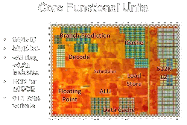
Therefore, if we want to duplicate the IPC we need to improve the superscalar hardware to analyze four time more instructions! Some hardware structures of the core such as fetching, or decoding will have to be scaled by a factor of four, but other structures need more aggressive scaling. For example to analyze the interdependences between two instruction we need only one comparison, because there is only one possible relationship between two any instructions, but increase the number of instructions to analyze to four and we need six comparisons –we have to compare the first instruction with the second instruction, the first with the third, the first with the fourth, the second with the third, the second with the fourth, and finally the third instruction with the fourth instruction–. For eight instructions the numbers of comparisons needed is twenty-eight. Detecting dependences among 2000 instructions requires almost two million comparisons! This cost obviously limits the number of instructions that can be considered for issue at once. Current cores have of the order of thousands of comparators.

This is not the only scaling problem. Code has branches, non-scientific code has a branch each eight or ten instructions. So, to fetch a sequence of hundreds of instructions the core must know, in advance, what paths will be taken on each bifurcation. This is the task of branch predictors. Imagine a predictor with average accuracy of 90%; this means that the prediction fails only in one branch of each ten. It can seem this very high accuracy solves the problem of branching in code, but accuracy reduces with each consecutive branch, because the probabilities of failed prediction increase with each new bifurcation. Consider a simple code example with only binary branches.

Whereas the probability the core is in the correct path after the first bifurcation point is of 90%, the probability that the core is in the correct path after the second branch is lower; the probability that the hardware correctly predicts the second branch continues being of 90%, but this probability is now bound to the probability of the core already being in the correct path after the first bifurcation. The probability the core is in the correct path after the second bifurcation point is now.

$$ \frac{90}{100}\frac{90}{100}=\frac{81}{100} $$

The probability has reduced to 81%. After ten consecutive binary branches the probability reduces to about 35%; this means the core is analyzing an incorrect sequence of instructions in two of three occasions! Current state-of-art predictors are very complex and include correlating tables for predictions; those tables keep a record of the paths taken by the core before and use those tables to improve the branch prediction by predicting a new branch in the context of the former branches leading up to it, instead predicting each branch just in isolation. Current state-of-art predictors are power-hungry and take up valuable space on the core.

One could think that being wrong in 5% of cases has a negligible impact on performance, but that is not correct. Things are not linear. When the core detect has been working in the incorrect path, it must cancel all the speculative work has been doing in advance, flush the pipeline entirely, and start again at the early point in the sequence of instructions where the prediction failed. This affect performance; this is called the mispredict branch penalty. Even with predictors accurate to 95%, the mispredict penalty can reduce the performance of a high-performance core by about one third. In other words, the core is not doing useful work one third of the time.

There are more scaling problems, and it is the reason why engineers hit an IPC wall. Indeed, if we plot the IPC per year for x86 processors, we get something like this:

The superscalar out-of-order microarchitectures behind the x86 ISA have hit a performance wall. No engineering team can break this wall, at best, engineers can spend years working on optimizing current microarchitectures to get a 2% IPC gain here and a 7% here. The only possibility to get a quantum jump on IPC over the current designs is if we change from a serial ISA, as x86, to a new ISA that scales up.

The existence of an IPC wall is not new. Research made decades ago about the limits of instruction level parallelism on code identified a soft wall about 10-wide cores. This wall was the reason why Intel engineers in collaboration with Hewlett Packard engineers developed a new ISA that would be scalable. The new ISA, dubbed EPIC, stands for Explicitly Parallel Instruction Computing. Intel wanted to use the migration from 32 bits to 64 bits to abandon x86 and replace it with EPIC. The plan failed badly because the promises of the new ISA could not be fulfilled. The reason? The ISA was developed around the concept of a smart compiler, which no one could build. Therefore, EPIC-based hardware was penalized by executing non-optimal binaries.

MYTH: GPUs performance grows faster than CPUs and soon GPUs will replace CPUs.

FACT: GPUs are easier to scale, but cannot replace CPUs.

Nvidia likes to share slides like this:

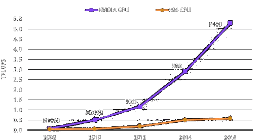
The evolution of GPUs is impressive, but the figure is measuring throughput. A GPU is an TCU (Throughput Compute Unit), whereas a CPU is a LCU (Latency Compute Unit); this is the terminology used by AMD in its HSA specification. GPUs are designed to crunch lots of numbers in a massively parallel way, when branches and the response time (latency) to changes are not relevant; otherwise a CPU is needed, this is the reason why GPUs are not used to execute the operative system.

Why are GPUs easier to scale up? Consider a process node shrink that provides four times higher density; for instance, a 14nm –> 7nm shrink. We could add four times more transistors in the same space. The key here is on how transistors are used in GPUs and CPUs. The relationship between IPC and number of transistors (the complexity of a microarchitecture) is not linear, but approximately given by.

$$ IPC=a\sqrt{A} $$

Where a is a parameter and A is the area used by transistors that execute a single thread. This is the so-called Pollack’s rule, which was derived empirically by him. For a theoretical derivation of the rule check this work by me.

Quadruplicating the number of transistors of a core will only produce a 100% increase in its IPC (we are assuming there is no other bottleneck in the system, and there is enough instruction level parallelism in the code). Alternatively, we could just build three more core identical to the original:

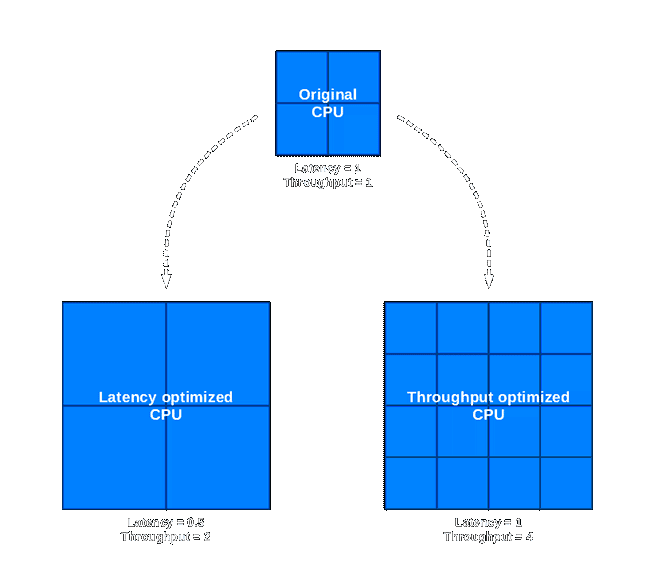
In the first case, the higher density provided by the new node has been used to increase the performance of each core by 100%; the total throughput has duplicated as well. In the second case, the higher density has been used to quadruplicate the total throughput. The same node shrink can give us two different performance increases; however, keep in mind that the twice higher throughput achieved by quadruplicating the number of cores does not come for free, because the latency is the same, whereas in the first case latency has also reduced by 100%.